Analysis for the Entertainment Channel

Maks Nikiforov and Mark Austin Due 10/31/2021

Data Import
Introduction
Summarizations
Modeling
Model Comparisons
References

##For markdown automation need a different 
##  image and cache folder 
##  for each of the 6 channels so that results
##    from different channels don't overwrite each other
##Also setting up currentChannel variable 
if (params$channel=="data_channel_is_bus") {
  knitr::opts_chunk$set(fig.path = "images/bus/",
                        cache.path = "cache/bus/")
  currentChannel<-"Business"
} else if (params$channel=="data_channel_is_entertainment") {
  knitr::opts_chunk$set(fig.path = "images/entertainment/",
                        cache.path="cache/entertainment/")
  currentChannel<-"Entertainment"
} else if (params$channel=="data_channel_is_lifestyle") {
  knitr::opts_chunk$set(fig.path = "images/lifestyle/",
                        cache.path = "cache/lifestyle/")
  currentChannel<-"Lifestyle"
} else if (params$channel=="data_channel_is_socmed") {
  knitr::opts_chunk$set(fig.path = "images/socmed/",
                        cache.path = "cache/socmed/")
  currentChannel<-"Social Media"
} else if (params$channel=="data_channel_is_tech") {
  knitr::opts_chunk$set(fig.path = "images/tech/",
                        cache.path = "cache/tech/")
  currentChannel<-"Tech"
} else if (params$channel=="data_channel_is_world") {
  knitr::opts_chunk$set(fig.path = "images/world/",
                        cache.path = "cache/world/")
  currentChannel<-"World"
} 

Data Import

Data was imported first to allow for a more automated introduction.

# Read all data into a tibble
fullData<-read_csv("./data/OnlineNewsPopularity.csv")

# Eliminate non-predictive variables
reduceVarsData<-fullData %>% select(-url,-timedelta)

#test code for pre markdown automation
#params$channel<-"data_channel_is_bus"

#filter by the current params channel
channelData<-reduceVarsData %>% filter(eval(as.name(params$channel))==1) 

# URL data for top ten articles in each category
channelDataURL <- fullData %>% filter(eval(as.name(params$channel))==1)

###Can now drop the data channel variables 
channelData<-channelData %>% select(-starts_with("data_channel"))

Introduction

This page offers an exploratory data analysis of Entertainment articles in the online news popularity data set. The top ten articles in this category, based on the number of shares on social media, include the following titles:

Shares	Article title
210300	Sprint’s New Plans Guarantee Unlimited Data for Life
197600	What to Do With Your New Xbox One
193400	McDonalds Kills Site That Advised Employees to Eat Healthy Meals
138700	How a $6,000 Video Got 6 Million Views and Launched a Business
112600	‘Flappy Bird Typing Tutor’ Is Even More Frustrating Than the Original
109500	Russian Hackers Used Microsoft Bug to Spy on Ukraine and NATO
109100	An App That Fights Back Against Smartphone Thieves
98500	Australian Patient Tests Negative for Ebola
98000	Facebook Makes Inroads in Russia With Yandex Partnership
96000	Samsung Trial Jury to Apple: Go After Google

Two variables - url and timedelta - are non-predictive and have been removed. The remaining 53 variables comprise 7057 observations, which makes up 17.8 percent of the original data set. Fernandes et al., who sourced the data, concentrated on article characteristics such as verbosity and the polarity of content, publication day, the quantity of included media, and keyword attributes (Fernandes et al., 2015). A subset of these variables and the correlations between them are explored in subsequent sections.

The broader purpose of this analysis is predicated on using supervised learning to predict a target variable - shares. To this end, the final sections outline four unique models for conducting such predictions and an assessment of their relative performance. Two models are rooted in multiple linear regression analysis, which assesses relationships between a response variable and two or more predictors. The remaining models are based on random forest and boosted tree techniques. The random forest method averages results from multiple decision trees which are fitted with a random parameter subset. The boosted tree method spurns averages in favor of results that stem from weighted iterations (James et al., 2021).

Summarizations

Numerical Summaries

The first table summarizes information for article shares grouped by whether an article was a weekend article or not. This summary gives an idea of the center and spread of shares across type of day group levels.

channelData %>% 
  mutate(dayType=ifelse(is_weekend,"Weekend","Weekday")) %>%
  group_by(dayType) %>% 
  summarise(Avg = mean(shares), Sd = sd(shares), 
    Median = median(shares), IQR =IQR(shares)) %>% kable()

dayType	Avg	Sd	Median	IQR
Weekday	2869.537	8059.543	1100	1102
Weekend	3647.273	6306.950	1650	2200

The next tables gives expands on the idea of the first table by grouping shares by each day of the week. This summary gives an idea of the center and spread of shares across day of the week group levels.

dowData<-channelData %>% select(starts_with("weekday_is"),shares) %>%
  mutate(dayofWeek=case_when(as.logical(weekday_is_monday)~"Monday",
                             as.logical(weekday_is_tuesday)~"Tuesday",
                             as.logical(weekday_is_wednesday)~"Wednesday",
                             as.logical(weekday_is_thursday)~"Thursday",
                             as.logical(weekday_is_friday)~"Friday",
                             as.logical(weekday_is_saturday)~"Saturday",
                             as.logical(weekday_is_sunday)~"Sunday")) %>%
  select(dayofWeek,shares)

dowLevels<-c("Monday","Tuesday","Wednesday",
             "Thursday","Friday","Saturday","Sunday")
dowData$dayofWeek<-factor(dowData$dayofWeek,levels = dowLevels)

dowData %>%  
  group_by(dayofWeek) %>% 
  summarise(Avg = mean(shares), Sd = sd(shares), 
    Median = median(shares), IQR =IQR(shares)) %>% kable()

dayofWeek	Avg	Sd	Median	IQR
Monday	2931.036	7176.296	1100	1102.0
Tuesday	2708.033	6453.317	1100	1115.0
Wednesday	2854.619	8285.402	1100	1131.5
Thursday	2882.213	9315.865	1100	1196.0
Friday	3000.947	9067.884	1200	1150.0
Saturday	3416.400	6459.886	1600	1400.0
Sunday	3810.951	6197.104	1700	2600.0

The table below highlights variables with the highest and most significant correlations in the data set. This output may be considered when analyzing covariance to control for potentially confounding variables.

# Display top 10 highest correlations
covarianceDF <- corr_cross(df = channelData, max_pvalue = 0.05, top = 10, plot = 0) %>% 
  select(key, mix, corr, pvalue) %>% rename("Variable 1" = key, "Variable 2" = mix, 
                                            "Correlation" = corr, "p-value" = pvalue) 

# Display non-zero p-values
covarianceDF[4] <- format.pval(covarianceDF[4])

kable(covarianceDF)

Variable 1	Variable 2	Correlation	p-value
n_unique_tokens	n_non_stop_unique_tokens	0.999973	< 2.22e-16
n_unique_tokens	n_non_stop_words	0.999920	< 2.22e-16
n_non_stop_words	n_non_stop_unique_tokens	0.999902	< 2.22e-16
kw_max_min	kw_avg_min	0.962390	< 2.22e-16
kw_min_min	kw_max_max	-0.867860	< 2.22e-16
LDA_01	LDA_03	-0.860914	< 2.22e-16
self_reference_max_shares	self_reference_avg_sharess	0.830012	< 2.22e-16
kw_max_avg	kw_avg_avg	0.821630	< 2.22e-16
global_rate_negative_words	rate_negative_words	0.790036	< 2.22e-16
weekday_is_sunday	is_weekend	0.742330	< 2.22e-16

Contingency Table

The following contingency table displays counts and sums for the number of article shares within given ranges by the day of week shared. Share ranges were selected to illustrate lower, medium, and higher ranges of shares. Examining these counts can show possible patterns of shares by day or week and the range grouping for shares.

##dig.lab is needed to avoid R defaulting to scientific notation
kable(addmargins(table
                 (dowData$dayofWeek,cut(dowData$shares,
                  c(0,200,1000,10000,860000),dig.lab = 7))))

	(0,200]	(200,1000]	(1000,10000]	(10000,860000]	Sum
Monday	6	619	655	78	1358
Tuesday	5	595	623	62	1285
Wednesday	5	627	596	67	1295
Thursday	4	570	594	63	1231
Friday	4	395	519	54	972
Saturday	2	65	287	26	380
Sunday	1	91	405	39	536
Sum	27	2962	3679	389	7057

Plots

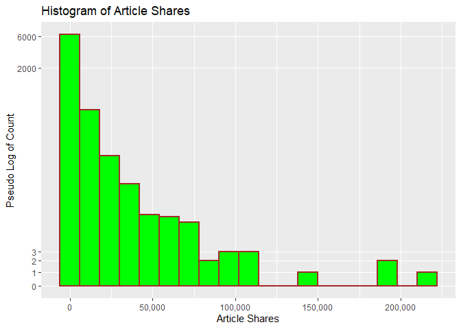
The following histogram looks at the distribution of shares. A pseudo log y scale with modified y break values was used so that article shares with low frequency will appear. We can tell from the histogram whether shares has a symmetric or skewed distribution. The distribution is symmetric if the tails are the same around the center. The distribution is right skewed if there is a long left tail and right skewed if there is a long right tail.

###creating histogram of shares data 
##scales comma was used to avoid the default scientific notation
##pseudo log with breaks was used to make low frequency values 
## more visisble
g <- ggplot(channelData, aes( x = shares))
g + geom_histogram(binwidth=12000,color = "brown", fill = "green", 
  size = 1)  + labs(x="Article Shares", y="Pseudo Log of Count",
  title = "Histogram of Article Shares") +
  scale_y_continuous(trans = "pseudo_log",
                     breaks = c(0:3, 2000, 6000),minor_breaks = NULL) +
  scale_x_continuous(labels = scales::comma) 

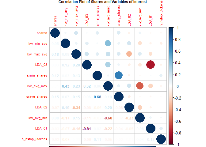
Fernandes et al. highlight several variables in their random forest model (Fernandes et al., 2015). The following variables from their top 11 were included in the following correlation plot with variables in () being renamed for this plot: shares,kw_min_avg,kw_max_avg,LDA_03,self_reference_min_shares(srmin_shares),kw_avg_max,self_reference_avg_sharess(sravg_shares),LDA_02,kw_avg_min,LDA_01,n_non_stop_unique_tokens(n_nstop_utokens).
The plot shows correlation with the response variable shares and the other various combinations. Larger circles indicate stronger positive (blue) or negative (red) correlation with correlation values on the lower portion of the plot.

##Reduce variable name length for later plotting
## Otherwise var names overwrite Title no matter
##  how many other size tweaks were made
corrData<-channelData %>% 
  mutate(sravg_shares=self_reference_avg_sharess,
         srmin_shares=self_reference_min_shares,
         n_nstop_utokens=n_non_stop_unique_tokens)

Correlation<-cor(select(corrData, shares, kw_min_avg,
        kw_max_avg, LDA_03, srmin_shares,
        kw_avg_max, sravg_shares, LDA_02,
        kw_avg_min, LDA_01, n_nstop_utokens),
        method = "spearman")

corrplot(Correlation,type="upper",tl.pos="lt", tl.cex = .70)
corrplot(Correlation,type="lower",method="number",
         add=TRUE,diag=FALSE,tl.pos="n",tl.cex = .70,number.cex = .75,
         title = 
           "Correlation Plot of Shares and Variables of Interest",
         mar=c(0,0,.50,0),cex.main = .75)

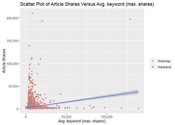
The following two scatterplots illustrate the relationship between response article shares shares and predictor average keyword (max shares) kw_max_ave. kw_max_ave was chosen because it was one of the potential predictors examined in the previous correlation plot.

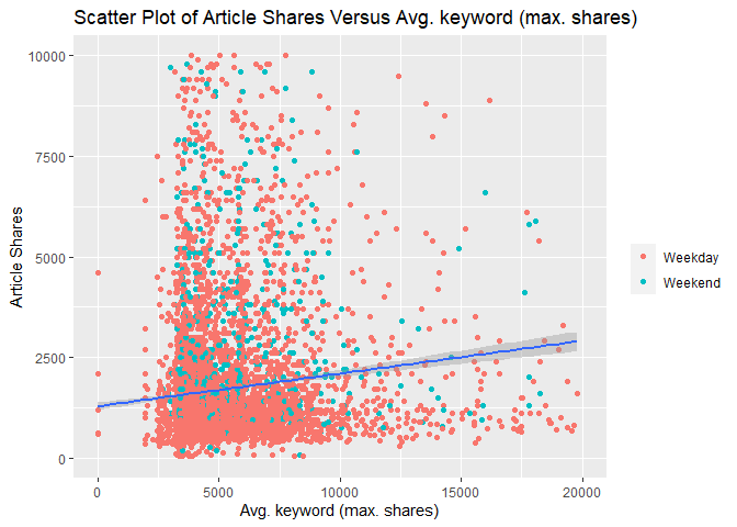
Both scatterplots plot these variables and add a simple linear regression line to the graph.

For either graph, an upward relationship indicates higher average keyword values tend towards more article shares. A negative relation would indicate a lower average keyword values tend towards more article shares.

In addition, both graphs use differing color for weekday and weekend articles so that we can spot any possible trends with those values too.

The first scatterplot uses the default R generated axes so that potential outliers or significant observations can be observed.

The second scatterplot reduces the scale of both axes to make it easier to spot relationships for the majority of data that occur within these bounds.

###Create new factor version of weekend variable 
### to use later in graphs
scatterData<-channelData %>% 
  mutate(dayType=ifelse(is_weekend,"Weekend","Weekday"))
scatterData$dayType<-as.factor(scatterData$dayType)

###First scatter plot with ALL data 
g<-ggplot(data = scatterData,
          aes(x= kw_max_avg,y=shares))
g + geom_point(aes(color=dayType)) +
  geom_smooth(method = lm) +
  scale_y_continuous(labels = scales::comma) +
  scale_x_continuous(labels = scales::comma) +
  labs(x="Avg. keyword (max. shares)", y="Article Shares",
       title = "Scatter Plot of Article Shares Versus Avg. keyword (max. shares)",color="") 

###Second scatter plot with reduced axes
g<-ggplot(data = scatterData,
          aes(x= kw_max_avg,y=shares))
g + geom_point(aes(color=dayType)) +
  geom_smooth(method = lm) +
  ylim(0,10000) +
  xlim(0,20000) +
    labs(x="Avg. keyword (max. shares)", y="Article Shares",
       title = "Scatter Plot of Article Shares Versus Avg. keyword (max. shares)",
       color="")

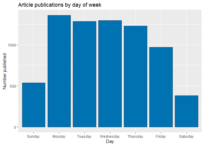
The bar plot below shows cumulative article publications for each day of the week, with higher bars indicating more publications. However, days with the largest number of publications are not necessarily ones with the most article shares, as seen in the subsequent box plot.

# Subset columns to include only weekday_is_*
weekdayData <- channelData %>% select(starts_with("weekday_is"))

# Calculate sum of articles published in each week day
articlesPublished <- lapply(weekdayData, function(c) sum(c=="1"))

# Use factor to set specific order in bar plot
weekPubDF <- data.frame(weekday=c("Monday", "Tuesday", "Wednesday", 
                           "Thursday", "Friday", "Saturday", "Sunday"),
                count=articlesPublished)
weekPubDF$weekday = factor(weekPubDF$weekday, levels = c("Sunday", "Monday", "Tuesday", "Wednesday", 
                           "Thursday", "Friday", "Saturday"))

# Create bar plot with total publications by day
weekdayBar <- ggplot(weekPubDF, aes(x = weekday, y = articlesPublished)) + geom_bar(stat = "identity", color = "#123456", fill = "#0072B2") 
weekdayBar + labs(x = "Day", y = "Number published",
       title = "Article publications by day of week")

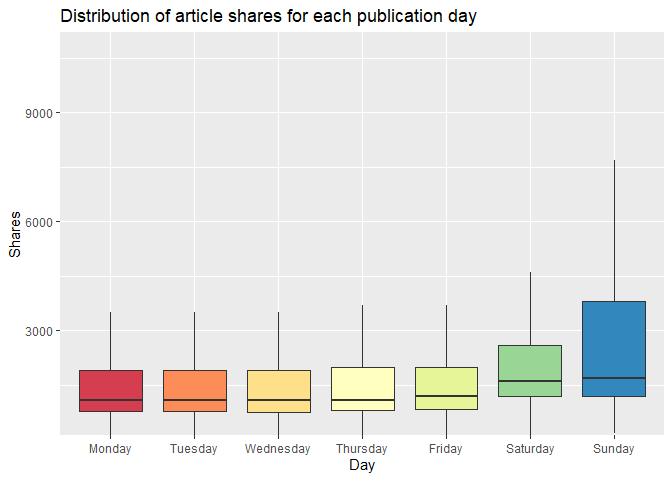
The boxplot below examines the day of article publication (Monday-Sunday) and the associated distribution of article shares. The median line indicates the center of the distribution of shares, and comparatively high medians indicate days that have relatively high circulation of Mashable articles in social media networks. For days in which the median is closer to the lower quartile (and where the upper whisker may be taller than the lower whisker), the distribution is skewed to the right. Conversely, a median that is closer to the upper quartile indicates a distribution that is skewed to the left. Days with relatively taller boxplots also have greater variability of shares.

# Subset columns to include only weekday_is_*, shares,
# create categorical variable, "day", denoting day of week (Mon-Sun)
medianShares <- channelData %>% select(starts_with("weekday_is"), shares) %>% mutate(day = NA)

# Populate "day"
for (i in 1:nrow(medianShares)) {
  if (medianShares$weekday_is_monday[i] == 1) {
    medianShares$day[i] = "Monday"
  }
  else if (medianShares$weekday_is_tuesday[i] == 1) {
    medianShares$day[i] = "Tuesday"
  }
  else if (medianShares$weekday_is_wednesday[i] == 1) {
    medianShares$day[i] = "Wednesday"
  }
  else if (medianShares$weekday_is_thursday[i] == 1) {
    medianShares$day[i] = "Thursday"
  }
  else if (medianShares$weekday_is_friday[i] == 1) {
    medianShares$day[i] = "Friday"
  }
  else if (medianShares$weekday_is_saturday[i] == 1) {
    medianShares$day[i] = "Saturday"
  }
  else if (medianShares$weekday_is_sunday[i] == 1) {
    medianShares$day[i] = "Sunday"
  }
  else {
    medianShares$day[i] = NA
  }
}

# Transform "day" into factor with levels to control order of boxplots
medianShares$day <- factor(medianShares$day, 
                           levels = c("Monday", "Tuesday", "Wednesday", 
                                      "Thursday", "Friday", "Saturday", "Sunday"))

# Plot distribution of shares for each day of the week
sharesBox <- ggplot(medianShares, aes(x = day, y = shares, fill = day))

sharesBox + geom_boxplot(outlier.shape = NA) + 
  # Exclude extreme outliers, limit range of y-axis
  coord_cartesian(ylim = quantile(medianShares$shares, c(0.1, 0.95))) +
  # Remove legend after coloration
  theme(legend.position = "none") +
  labs(x = "Day", y = "Shares",
       title = "Distribution of article shares for each publication day") + scale_fill_brewer(palette = "Spectral")

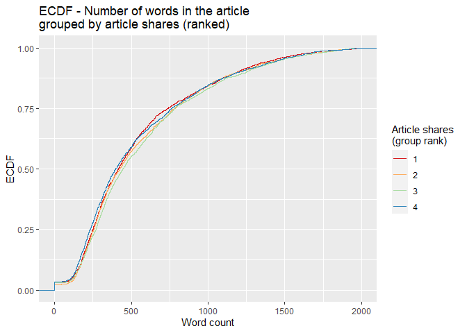
For the empirical cumulative distribution function (ECDF) below, the dplyr ranking function ntile() divides shares into four groups. Observations with the fewest shares are placed into group 1, those with the most shares are placed into group 4, and intermediaries reside in groups 2 and 3. The horizontal axis lists word count, and the vertical axis lists the percentage of content with that word count. A divergence of the colored lines suggests that the number of words differs in content with the fewest and most shares. At any given percentage of content (y-value), curves further to the right correspond to more words within the associated shares group. Groups with curves that are further to the left indicate fewer words in that percentage of content.

# Create variable to for binning the shares
binnedShares <- channelData %>% mutate(shareQuantile = ntile(channelData$shares, 4))
binnedShares <- binnedShares %>% mutate(totalMedia = num_imgs + num_videos)

# Render and label word count ECDF, group by binned shares
avgWordHisto <- ggplot(binnedShares, aes(x = n_tokens_content, colour = shareQuantile))
avgWordHisto + stat_ecdf(geom = "step", aes(color = as.character(shareQuantile))) +
  labs(title="ECDF - Number of words in the article \ngrouped by article shares (ranked)",
     y = "ECDF", x="Word count") + xlim(0,2000) + 
  scale_colour_brewer(palette = "Spectral", name = "Article shares \n(group rank)")

Modeling

Splitting Data

Per project requirements, the data for each channel are split with 70% of the data becoming training data and 30% of the data becoming test data.

#Using set.seed per suggestion so that work will be reproducible
set.seed(20)

dataIndex <-createDataPartition(channelData$shares, p = 0.7, list = FALSE)

channelTrain <-channelData[dataIndex,]
channelTest <-channelData[-dataIndex,]

Linear Regression Models

Linear regression models describe a linear relationship between a response variable and one or more explanatory variables. Models with one explanatory variable are called simple linear regression models and models with more than one explanatory variable are called multiple linear regression models. Multiple linear regression models can include polynomial and interaction terms. Each explanatory variable has an associated estimated parameter. All linear regression models are linear in the parameters.

For linear regression, explanatory variables can be continuous or categorical. However, response variables are only continuous for linear regression models.

Linear regression models are fit with training data by minimizing the sum of squared errors. Model fitting results in a line for simple linear regression and a saddle for multiple linear regression.

The first linear regression model contains predictors that encompass content keywords, sentiment and subjectivity, the length of content (the effects of which were gleaned previously from the ECDF), and link citations.

# Parallel cluster setup
cl <- makePSOCKcluster(6)
registerDoParallel(cl)

# Linear regression with subset of predictors (p-value < 0.1) selected after performing 
# least squares fit on the entire set of predictors. 
lmFit1 <- train(shares ~ kw_avg_avg + kw_max_avg + kw_min_avg + 
    num_hrefs + self_reference_min_shares + global_subjectivity + 
    num_self_hrefs + n_tokens_title + n_tokens_content + n_unique_tokens + 
    average_token_length + kw_min_max + num_keywords + kw_max_min + abs_title_subjectivity + 
    global_rate_positive_words, 
    data = channelTrain,
               method = "lm",
               preProcess = c("center", "scale"),
               trControl = trainControl(method = "cv", 
                                        number = 5))
stopCluster(cl)

The second linear regression model contains main effects for most of the predictors listed earlier in the correlation plot. If variables had more than .50 pairwise correlation in any channel, one variable of that pair was excluded. Excluded variables were: self_reference_min_shares, kw_avg_max, and LDA_01.

cl <- makePSOCKcluster(6)
registerDoParallel(cl)

lmFit2 <- train(shares ~ kw_min_avg +
        kw_max_avg + LDA_03 +  
        self_reference_avg_sharess + LDA_02 +
        kw_avg_min + n_non_stop_unique_tokens, 
               data = channelTrain,
               method = "lm",
               preProcess = c("center", "scale"),
               trControl = trainControl(method = "cv", 
                                        number = 10))


stopCluster(cl)

Random Forest Model

Random forest models aggregate results from many sample decision trees. Those sample trees are produced using bootstrap samples created using resampling with replacement. A tree is trained on each bootstrap sample, resulting in a prediction based on that training sample data. Results from all bootstrap samples are averaged to arrive at a final prediction.

Both bagging and random forest methods use bootstrap sampling with decision trees. However, bagging includes all predictors which can lead to less reduction in variance when strong predictors exist. Unlike bagging, random forests do not use all predictors but use a random subset of predictors for each bootstrap tree fit. Random forests usually have a better fit than bagging models.

In this particular case, the response shares is continuous and we are working with regression trees. The mtry tuning parameter controls how many random predictors are used in the bootstrap samples. An mtry of 1 to 30 was chosen as a way to evaluate up to 30 predictors. These values were chosen to work within available computing constraints. Five fold cross validation is used to choose the optimal mtry value corresponding to the lowest RMSE.

##Run time presented a challenge so parallel processing was used
##Followed Parallel instructions on caret page
##   https://topepo.github.io/caret/parallel-processing.html

##Various mtry values were tried with a 20 minute runtime goal
##  A 20 minute per channel runtime corresponds 
##  to a total of about 2 hours model fit for all 6 channels

##mtry 1:30 was chosen because it was close to 20 minutes
##mtry 1:20 had 10 minute runtime and 1:30 took 30 minutes

##repeatedcv was evaluated but took over 30 minutes 
## thus repeats were not used


cl <- makePSOCKcluster(6)
registerDoParallel(cl)

rfFit <- train(shares ~ ., data = channelTrain,
               method = "rf",
               preProcess = c("center", "scale"),
               trControl = trainControl(method = "cv",
                                number = 5),
               tuneGrid = data.frame(mtry = 1:30))

stopCluster(cl)

rfFit

## Random Forest 
## 
## 4941 samples
##   52 predictor
## 
## Pre-processing: centered (52), scaled (52) 
## Resampling: Cross-Validated (5 fold) 
## Summary of sample sizes: 3953, 3952, 3952, 3954, 3953 
## Resampling results across tuning parameters:
## 
##   mtry  RMSE      Rsquared    MAE     
##    1    8146.052  0.01887343  3096.448
##    2    8174.125  0.02203567  3169.326
##    3    8235.135  0.02136987  3217.389
##    4    8266.471  0.02003954  3242.563
##    5    8313.914  0.02036114  3262.135
##    6    8337.857  0.02066536  3282.867
##    7    8352.204  0.02193915  3287.158
##    8    8419.087  0.01959036  3314.204
##    9    8451.066  0.01869157  3316.410
##   10    8465.114  0.01875888  3326.554
##   11    8498.379  0.01749859  3341.798
##   12    8529.930  0.01734652  3355.287
##   13    8543.489  0.01647041  3357.204
##   14    8556.173  0.01811867  3366.488
##   15    8553.460  0.01726190  3366.237
##   16    8575.025  0.01852606  3366.201
##   17    8594.662  0.01778448  3369.376
##   18    8589.616  0.01715711  3385.373
##   19    8645.761  0.01658968  3393.000
##   20    8647.892  0.01789295  3403.785
##   21    8635.030  0.01668729  3401.357
##   22    8651.967  0.01596879  3409.186
##   23    8689.784  0.01628225  3412.077
##   24    8641.716  0.01566695  3403.957
##   25    8696.739  0.01533226  3417.636
##   26    8694.429  0.01710042  3423.940
##   27    8691.298  0.01644809  3415.688
##   28    8728.543  0.01693086  3431.457
##   29    8771.681  0.01489720  3432.953
##   30    8804.943  0.01486717  3449.670
## 
## RMSE was used to select the optimal model using the smallest value.
## The final value used for the model was mtry = 1.

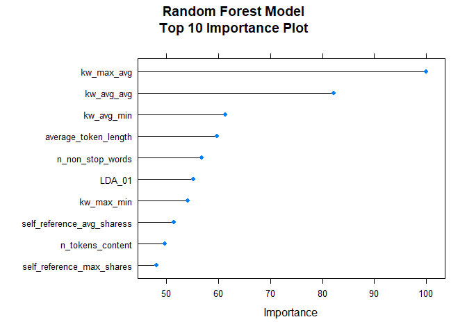
After fitting the random forest model, the following variable importance plot is created. The top ten most important predictors are plotted using a scale of 0 to 100.

rfImp <- varImp(rfFit, scale = TRUE)
plot(rfImp,top = 10, main="Random Forest Model\nTop 10 Importance Plot")

Boosted Tree Model

Boosting is a general method whereby decision trees are grown sequentially using residuals (the differences between observed values and predicted values of a variable) as the response. Initial prediction values start at 0 for all combinations of predictors, so that the first set of residuals matches the observed values in our data. To mitigate low bias and high variance, contributions from subsequent trees are scaled with a shrinkage parameter, λ. The value of this parameter is generally small (0.01 or 0.001), which slows tree growth and tampers overfitting (James et al., 2021).

# Re-allocate cores for parallel computing
cl <- makePSOCKcluster(6)
registerDoParallel(cl)


# Boosted tree fit with tuneLength (let function decide parameter combinations)
boostedTreeFit <- train(shares ~ ., data = channelTrain,
               method = "gbm",
               preProcess = c("center", "scale"),
               trControl = trainControl(method = "cv", 
                                        number = 5),  
               tuneLength = 5)

## Iter   TrainDeviance   ValidDeviance   StepSize   Improve
##      1 74291104.4915             nan     0.1000 192788.3110
##      2 73687107.5229             nan     0.1000 109723.2721
##      3 73149568.9716             nan     0.1000 -51921.1454
##      4 72789874.3741             nan     0.1000 95810.3338
##      5 72246793.6662             nan     0.1000 358281.6201
##      6 71605249.1859             nan     0.1000 -186499.8001
##      7 71308396.6790             nan     0.1000 49202.5007
##      8 70934901.4538             nan     0.1000 31971.2775
##      9 70244531.8704             nan     0.1000 230940.3674
##     10 69974110.0579             nan     0.1000 -173304.1494
##     20 68186626.4804             nan     0.1000 -233191.9307
##     40 65180740.3046             nan     0.1000 -514442.2699
##     50 63885285.0550             nan     0.1000 -125671.1932

# Define tuning parameters based on $bestTune from the permutations above
nTrees <- boostedTreeFit$bestTune$n.trees
interactionDepth = boostedTreeFit$bestTune$interaction.depth
minObs = boostedTreeFit$bestTune$n.minobsinnode
shrinkParam <- boostedTreeFit$bestTune$shrinkage

# Boosted tree fit with defined parameters
bestBoostedTree <- train(shares ~ ., data = channelTrain,
               method = "gbm",
               preProcess = c("center", "scale"),
               trControl = trainControl(method = "cv", 
                                        number = 5),  
               tuneGrid = expand.grid(n.trees = nTrees, interaction.depth = interactionDepth,
                                      shrinkage = shrinkParam, n.minobsinnode = minObs))

## Iter   TrainDeviance   ValidDeviance   StepSize   Improve
##      1 74529726.6283             nan     0.1000 257718.1361
##      2 74093939.1404             nan     0.1000 387301.4818
##      3 73603711.7175             nan     0.1000 182634.4991
##      4 73176710.5652             nan     0.1000 69362.1274
##      5 72854614.6397             nan     0.1000 -5083.6528
##      6 72586638.0497             nan     0.1000 21545.3920
##      7 71948667.2515             nan     0.1000 -10432.0240
##      8 71718045.6386             nan     0.1000 -267218.3958
##      9 70873329.9144             nan     0.1000 410397.3030
##     10 70243828.4588             nan     0.1000 -235128.4592
##     20 67405493.6449             nan     0.1000 -190842.2488
##     40 64101417.8058             nan     0.1000 -119653.4839
##     50 62930988.3505             nan     0.1000 -313439.9645

stopCluster(cl)

Model Comparisons

After models were fit with training data, we do predictions with testing data. Finally, RMSE metrics are extracted and compared. The model with lowest RMSE is presented as the winning model.

# Predict using test data
predictLM1 <- predict(lmFit1, newdata = channelTest)

# Metrics
RMSELM1 <- postResample(predictLM1, obs = channelTest$shares)["RMSE"][[1]]
RMSELM1

## [1] 5542.229

# Store value for model comparison
modelPerformance <- tibble(RMSE = RMSELM1, Model = "Linear regression 1")

predictLM2 <- predict(lmFit2, newdata = channelTest)
RMSELM2<-postResample(predictLM2, channelTest$shares)["RMSE"][[1]]
RMSELM2

## [1] 5518.04

modelPerformance <- add_row(modelPerformance, RMSE = RMSELM2, Model = "Linear regression 2")

predictRF <- predict(rfFit, newdata = channelTest)
RMSERF<-postResample(predictRF, channelTest$shares)["RMSE"]
RMSERF

##     RMSE 
## 5389.443

modelPerformance <- add_row(modelPerformance, RMSE = RMSERF, Model = "Random forest")

# Predict using test data
predictGBM <- predict(bestBoostedTree, newdata = channelTest)

# Metrics
RMSEGBM <- postResample(predictGBM, obs = channelTest$shares)["RMSE"]
RMSEGBM

##     RMSE 
## 5591.718

modelPerformance <- add_row(modelPerformance, RMSE = RMSEGBM, Model = "Boosted tree")

# Select row with lowest value of RMSE.
selectModel <- modelPerformance %>% slice_min(RMSE)
selectModel

## # A tibble: 1 x 2
##    RMSE Model        
##   <dbl> <chr>        
## 1 5389. Random forest

Based on the preceding analyses with test data, the Random forest model yields the lowest RMSE - 5389.4434873.

References

Fernandes, K., Vinagre, P., & Cortez, P. (2015). A proactive intelligent decision support system for predicting the popularity of online news. In F. Pereira, P. Machado, E. Costa, & A. Cardoso (Eds.), *Progress in artificial intelligence* (pp. 535–546). Springer International Publishing.

James, G., Witten, D., Hastie, T., & Tibshirani, R. (2021). *An introduction to statistical learning*. Springer US. <https://doi.org/10.1007/978-1-0716-1418-1>